Frank-Wolfe¶

Note from Editors

This article has been flagged as incomplete for the following:

Incomplete / poorly formatted list of properties
Inadequate references to applications (Section: Applications)
Inadequate references to related works (Section: See Also)

Definition¶

For a constraint set \(\mathcal{C} \subseteq \mathbb{H}\)¹ and a function² \(\ \mathsf{f\colon \mathbb{H} \rightarrow \overline{\mathbb{R}}}\) that is differentiable over \(\mathcal{C}\), consider the constrained minimization problem

\[ \mathsf{\underset{x \in \mathcal{C}}{min} \ f(x).} \]

Frank-Wolfe is an iterative scheme for solving this problem with update \(\mathsf{x^{k+1}}\) defined by

\[\begin{aligned} \mathsf{s^{k+1}} & \mathsf{\triangleq \underset{x\in \mathcal{C}}{argmin} \ \left< \nabla f(x^k),\ x \right>, } \\ \mathsf{x^{k+1}} & \mathsf{\triangleq x^k + \alpha_k \left( s^{k+1} - x^k \right),} \end{aligned}\]

with a step size rule typically given by either

\[ \mathsf{\alpha_k = \dfrac{2}{k+2} \quad {or} \quad \alpha_k = \underset{\alpha\in[0,1]}{argmin} \ f\left(x^k + \alpha (s^k - x^k)\right).} \]

Overview¶

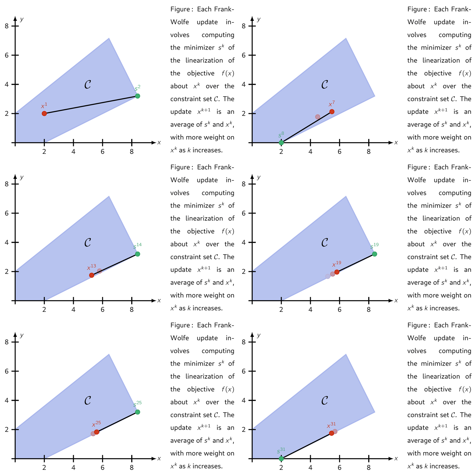
The Frank–Wolfe (FW) algorithm, also called "conditional gradient", is an iterative first-order algorithm for solving constrained convex problems. The method was proposed by Marguerite Frank and Philip Wolfe in 1956.³ Each update is a convex combination between the current iterate \(\mathsf{x^k}\) and a minimimizer \(\mathsf{s^k}\) of the linearization of \(\mathsf{f}\) about \(\mathsf{x^k}\) over the domain \(\mathcal{C}\). This ensures each iteration is feasible. Several standard convergence properties hold for FW and its variants.

Illustration¶

Consider the problem

\[\mathsf{\min_{x \in \mathbb{R}^2} \dfrac{1}{2} \left\|x-\left[\begin{array}{c} \mathsf{6} \\ \mathsf{1}\end{array}\right] \right\|^2 \ \ \ \mbox{s.t.}\ \ \ \left[\begin{array}{rr} \mathsf{2} & \mathsf{1} \\ \mathsf{-4} & \mathsf{5} \\ \mathsf{1} & \mathsf{-2}\end{array}\right]x \leq \left[\begin{array}{c} \mathsf{20} \\ \mathsf{10} \\ \mathsf{2} \end{array}\right],\ \ x\geq 0.}\]

Letting the set of feasible solutions be denoted by \(\mathcal{C}\), below is an illustration of applying Frank-Wolfe with step-size \(\mathsf{\alpha_k = 2 / (k + 2)}.\)

grahpic-fw

Properties¶

Convergence Theorem⁴

If \(\mathsf{f}\) is convex and Lipschitz differentiable over a convex and compact set \(\mathcal{C}\), then there is a constant \(\mathsf{C> 0}\) such that

\[ \mathsf{f(x^k) \leq f(x^\star) + \dfrac{C}{k+2},} \]

where \(\mathsf{x^\star}\) is a minimizer of \(\mathsf{f}\) over \(\mathcal{C}\).

Zigzag Behavior⁵

Oscillations can occur...

Invariant to Coordinate System⁶

Can rescale or re-jigger coordinates without any change in outcomes.

Feasible + Projection-Free

No projections needed if \(\mathsf{x^1 \in \mathcal{C}.}\)

Code¶

Python (Linear Constraints)Python (Illustration)

    from scipy.optimize import linprog
    import numpy as np 

    def frankWolfe(grad, x_init, A_eq, b_eq, A_ineq, b_ineq,
                   bnds, tol=1.0e-6):
    ''' Minimize function subject to inequality constraints

        Args:
            grad:   function for gradient of cost 
            x_init: initial estimate
            A_eq:   matrix for equality constraint
            b_eq:   vector for equality constraint
            A_ineq: matrix for inequality constraint
            b_ineq: vector for inequality constraint  
            bnds:   box constraint bounds   
        Returns:
            x: solution estimate
    '''
    k = 1.0  
    x = x_init.copy() 
    converge = False
    while not converge: 
        c   = grad(x).transpose()
        opt = linprog(c=c, A_ub=A_ineq, b_ub=b_ineq,
                      A_eq=A_eq, b_eq=b_eq, bounds=bnds)
        s     = np.reshape(opt.x, x.shape)
        alpha = 2.0 / (k + 2.0)
        step  = alpha * (s - x)              
        x    += step
        k    += 1.0
        converge = np.linalg.norm(step) <= tol 
    return x

    lhs_ineq = [[ 2,  1], [-4,  5], [1, -2]]  
    rhs_ineq = [20, 10, 2]
    bnd      = [(0, float("inf")), (0, float("inf"))]
    ref      = np.array([[6.0], [1.0]])
    x_init   = np.array([[2.0], [2.0]])

    def grad(x):
        """ Compute gradient of 0.5 * || x - ref || ** 2
        """
        return x - ref

    sol = frankWolfe(grad, x_init, None, lhs_ineq, None,
                     rhs_ineq, bnd)

Applications¶

Statistics.
Compressed sensing.